RelDists, DiscreteDists and RealDists
New distributions to complement GAMLSS regression models
Universidad de Antioquia-Colombia , Universidad Nacional de Colombia-Colombia
September 18, 2024
Slides available at

RelDists, DiscreteDists and RealDists
How these packages fit into R and the statistical literature?
Linear Models
\[\begin{align} Y_i &\sim N(\mu_i, \sigma^2), \\ \mu_i &= \beta_0 + \beta_1 X_{1i} + \beta_2 X_{2i} + \cdots + \beta_p X_{pi}, \\ \sigma^2 &= \text{constant}. \end{align}\]Generalized linear models
\[\begin{align} Y_i &\sim D(\mu_i, \phi), \\ g(\mu_i) &= \beta_0 + \beta_1 X_{1i} + \beta_2 X_{2i} + \cdots + \beta_p X_{pi}, \\ \phi &= \text{constant}. \end{align}\]The distribution \(D\) can be: Normal, Binomial, Negative Binomial, Poisson, Gamma and Inverse gaussian.
GAMLSS: Generalized Additive Models for Location, Scale and Shape
\[\begin{align} Y_i &\sim D(\mu_i, \sigma_i, \nu_i, \tau_i), \\ g_1(\mu_i) &= \beta_{10} + \beta_{11} X_{1i} + \beta_{12} X_{2i} + \cdots + \beta_{1p} X_{pi}, \\ g_2(\sigma_i) &= \beta_{20} + \beta_{21} X_{1i} + \beta_{22} X_{2i} + \cdots + \beta_{2p} X_{pi}, \\ g_3(\nu_i) &= \beta_{30} + \beta_{31} X_{1i} + \beta_{32} X_{2i} + \cdots + \beta_{3p} X_{pi}, \\ g_4(\tau_i) &= \beta_{40} + \beta_{41} X_{1i} + \beta_{42} X_{2i} + \cdots + \beta_{4p} X_{pi}. \end{align}\]The distribution \(D\) can be: Normal, Binomial, Negative Binomial, Poisson, Gamma and Inverse gaussian, Weibull, beta, ZIP, ….
GAMLSS: Generalized Additive Models for Location, Scale and Shape
More details about gamlss in https://www.gamlss.com.

RelDists
Distributions
Thirty distributions were implemented in the RelDists package. Some of these distributions are:
- Additive Weibull
AddW. - Beta Generalized Exponentiated
BGE. - Cosine Sine Exponential
CS2e. - Extended Exponential Geometric
EEG. - Flexible Weibull Extension
FWE. - …
The complete list can be found at this link.
Functions
Each distribution has the following functions:
XXX: It refers to the short name of the distribution.
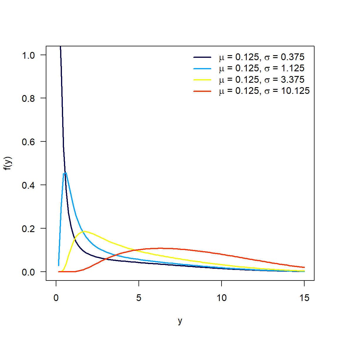
Flexible Weibull Extension (FWE)
This distribution was proposed by Bebbington (2007) and its density function is given by the following expression:
\[ f(y; \mu, \sigma) = \left( \mu+ \frac{\sigma}{y^2} \right) e^{\mu y - \sigma / y} \exp \left( -e^{\mu y - \sigma / y} \right), \]
with \(\mu > 0\), \(\sigma > 0\), \(y>0\).
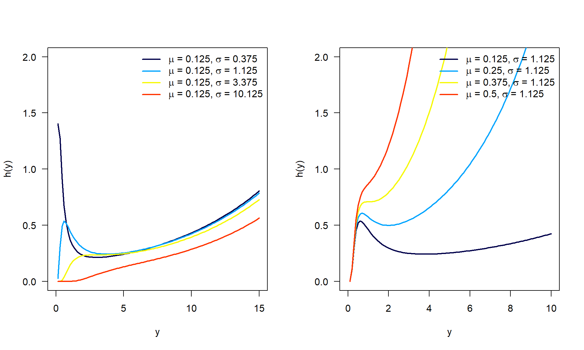
Flexible Weibull Extension (FWE)
The hazard function of the FWE distribution has great flexibility and it is given by:
\[h(y) = \left( \mu+ \frac\sigma{y^2} \right) e^{\mu y - \sigma / y}.\]
Probability density function
Hazard function
Example 1
n <- 100
mu <- 0.75
sigma <- 1.3

library(RelDists)
set.seed(123)
y <- rFWE(n=n, mu, sigma)

library(gamlss)
mod <- gamlss(y~1, sigma.fo=~1, family="FWE", control=gamlss.control(trace=FALSE))

exp(coef(mod, what="mu"))
(Intercept)
0.7776793 (Intercept)
1.331533 The estimates are close to the real values 🙏.
Example 2
n <- 200
library(RelDists)
set.seed(123)
{
  x1 <- runif(n)
  x2 <- runif(n)
  mu <- exp(1.21 - 3 * x1)
  sigma <- exp(1.26 - 2 * x2)
  y <- rFWE(n=n, mu, sigma)
}

library(gamlss)
mod <- gamlss(y~x1, sigma.fo=~x2, family=FWE, control=gamlss.control(trace=FALSE))

coef(mod, what="mu")
(Intercept) x1
1.131260 -2.831916 (Intercept) x2
1.305884 -2.063528 DiscreteDists
Distributions
Nine distributions were implemented in the DiscreteDists package. Some of these distributions are:
- Discrete Burr Hatke
DBH. - Discrete generalized exponential
DGEII. - Discrete Inverted Kumaraswamy
DIKUM. - Discrete Lindley
DLD. - Discrete Generalized Exponential II
DGEII. - …
The complete list can be found at this link.
Functions
Each distribution has the following functions:
XXX: It refers to the short name of the distribution.
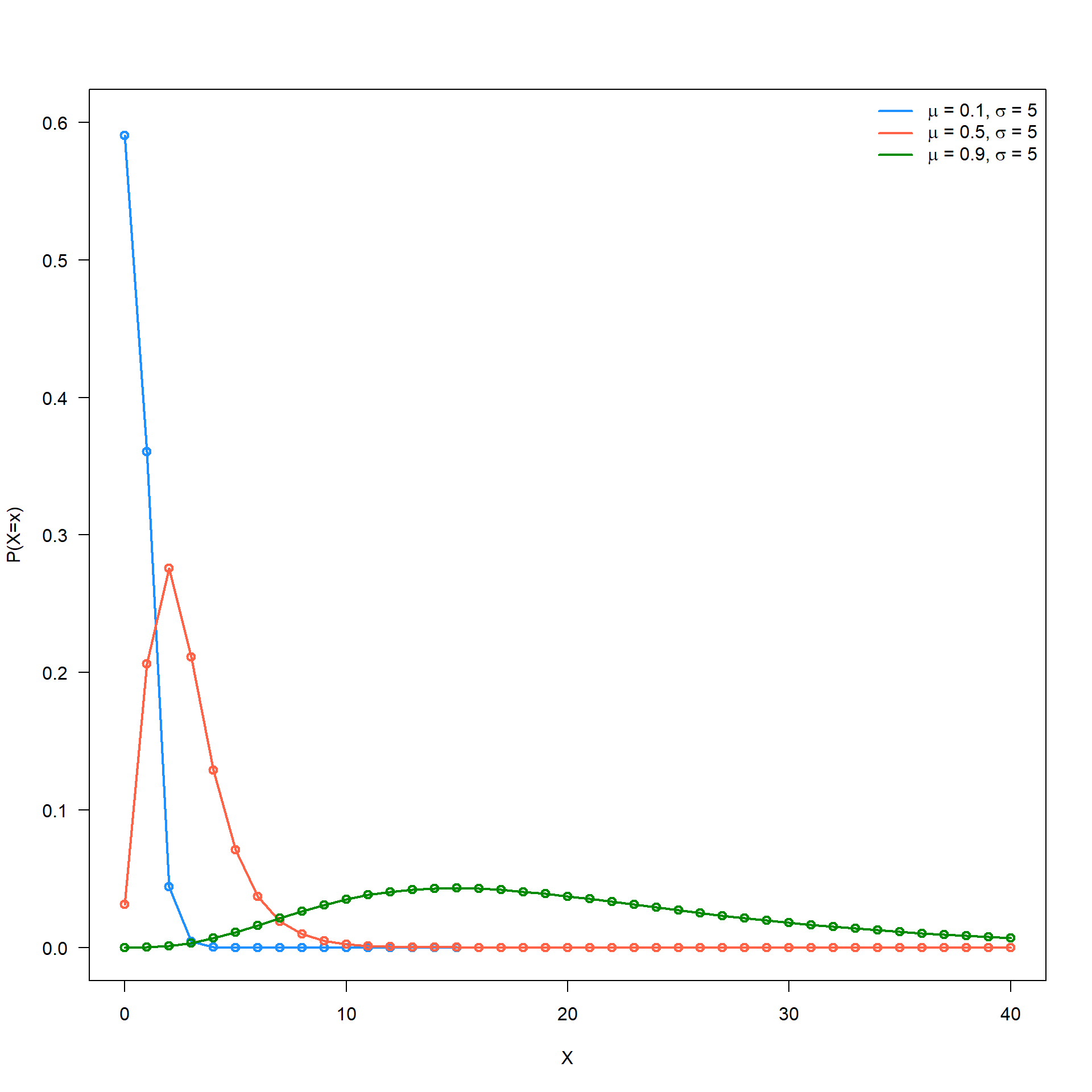
Discrete Generalized Exponential Distribution
The Discrete Generalized Exponential Distribution (DGEII) distribution with parameters \(\mu\) and \(\sigma\) has a support \(0, 1, 2, ...\) and mass function given by
\[ 𝑓(𝑥|𝜇,𝜎)=(1−𝜇𝑥+1)𝜎−(1−𝜇𝑥)𝜎, \]
with \(0<\mu<1\) and \(\sigma>0\). If \(\sigma=1\), the DGEII distribution reduces to the geometric distribution with success probability \(1−\mu\).
Mass probability function
Example
n <- 100
mu <- 0.75
sigma <- 0.5

library(DiscreteDists)
set.seed(123)
y <- rDGEII(n = n, mu, sigma)

library(gamlss)
mod <- gamlss(y~1, family=DGEII, control=gamlss.control(n.cyc=500, trace=FALSE))

inv_logit <- function(x) 1/(1 + exp(-x))
inv_logit(coef(mod, what="mu"))
(Intercept)
0.7472655 (Intercept)
0.4681355 RealDists
Distributions
One distribution was implemented in the RealDists package:
- Generalised exponential-Gaussian
GEG.
The package can be found at this link.
Functions
The distribution has the following functions:
XXX: It refers to the short name of the distribution.
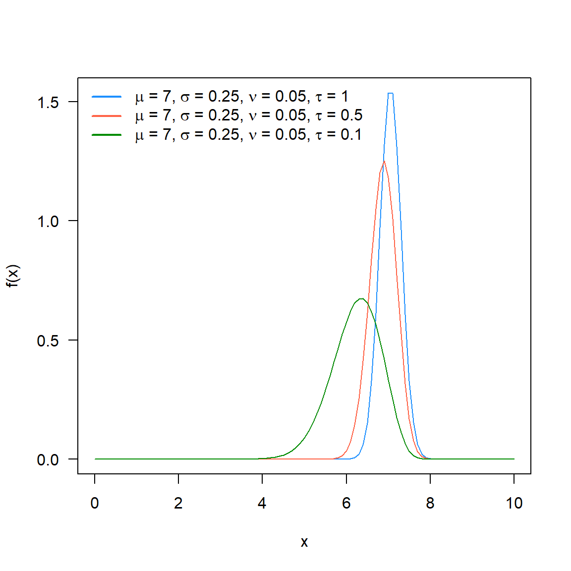
Generalised exponential-Gaussian
The Generalised exponential-Gaussian with parameters \(\mu, \sigma, \nu\) and \(\tau\) has density given by
\[ 𝑓(𝑥|𝜇,𝜎,𝜈,𝜏)=\frac{𝜏}{𝜈}\exp(𝑤)Φ\left(𝑧−\frac{𝜎}{𝜈}\right)\left[Φ(𝑧)−\exp(𝑤)Φ\left(𝑧−\frac{𝜎}{𝜈}\right)\right]^{𝜏−1}, \]
for \(−∞<𝑥<∞\). With \(𝑤=\frac{𝜇−𝑥}{𝜈}+\frac{\sigma^2}{2\nu^2}\) and \(𝑧=\frac{𝑥−𝜇}{𝜎}\) and \(Φ\) is the cumulative function for the standard normal distribution.
Density probability function
Example
n <- 500
mu <- -5 ; sigma <- 4 ; nu <- 2.5 ; tau <- 1

library(RealDists)
set.seed(123)
y <- rGEG(n=n, mu, sigma, nu, tau)

library(gamlss)
mod <- gamlss(y ~ 1, family=GEG, control=gamlss.control(n.cyc=1000, trace=FALSE))

coef(mod, what="mu")
(Intercept)
-5.918508 (Intercept)
3.725721 (Intercept)
2.978824 (Intercept)
1.116511 Final comments
These new R packages allow:
Use the functions dXXX(), pXXX(), qXXX(), and rXXX().
Estimate distribution parameters and regression model parameters can be estimated.
Integrate the new distributions into their statistical analyses.
Future work
If you want to be part of the team that develops these packages, please write to us at: fhernanb@unal.edu.co and olga.usuga@udea.edu.co.

Conference

Conference


COBIPE - 1º Colóquio Binacional Brasil-Colômbia de Probabilidade e Estatística